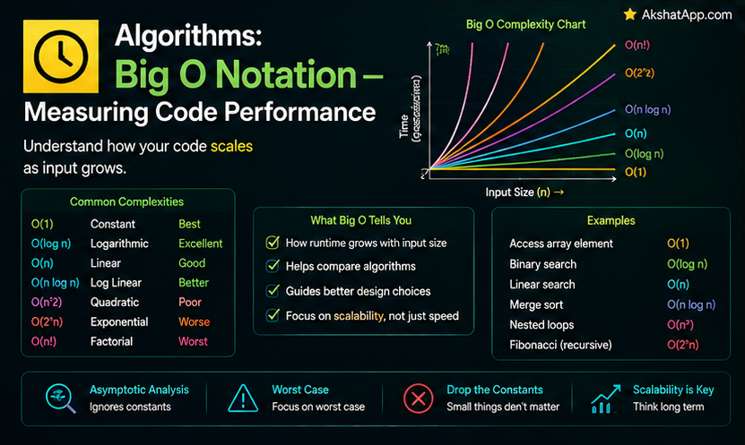
Post #4 called hash table access “O(1) average case.” Post #5 called BST search “O(log n)” for a balanced tree. Post #3 called array indexing “O(1)” and inserting into the middle of an array “O(n).” Every one of these claims has been used without a formal definition, on the promise that this post would make them precise. This is that post — and because every example in it is already familiar from earlier in this series, Big O notation should land as a natural, useful formalization of intuitions you already have, not new abstract theory.
What Big O Actually Measures
Big O describes how an algorithm’s resource usage — almost always time, sometimes memory — grows as the input size grows, not the exact number of seconds or operations a specific run takes. This distinction matters enormously: the exact runtime depends on your specific CPU (Post #1), how the code is written, and countless other factors — but the growth rate as input size increases is a genuine, mathematical property of the algorithm itself, independent of any of that.
def find_max(numbers: list[int]) -> int:
    current_max = numbers[0]
    for n in numbers:
        if n > current_max:
            current_max = n
    return current_max
This function examines every element exactly once. Double the input size, and the work roughly doubles too — this growth pattern, “work scales linearly with input size,” is what Big O calls O(n), regardless of whether your specific machine happens to complete it in one millisecond or one microsecond.
The Common Complexity Classes, With Examples Already Familiar From This Series
O(1) — Constant Time
Work stays the same regardless of input size.
def get_first(items: list) -> any:
    return items[0]  # always exactly one operation, whether items has 3 elements or 3 million
Already covered in this series: Post #3’s array indexing (array[5]) and Post #4’s hash table lookup (dict[key]) are both O(1) — the defining reason both structures felt so fast in those earlier posts.
O(log n) — Logarithmic Time
Work grows, but very slowly — each doubling of input size adds only one more unit of work.
def bst_search(node, value):
    if node is None or node.value == value:
        return node
    elif value < node.value:
        return bst_search(node.left, value)
    else:
        return bst_search(node.right, value)
Already covered in this series: Post #5’s balanced BST search — every comparison eliminates half the remaining tree, exactly the “halving” pattern that produces logarithmic growth.
O(n) — Linear Time
Work grows directly proportional to input size — this post’s opening find_max example.
Already covered in this series: Post #3’s linked list traversal to reach a specific position; Post #5’s in-order tree traversal, visiting every node exactly once.
O(n log n) — Linearithmic Time
A very common, genuinely efficient pattern for algorithms that divide the problem repeatedly (the log n part) but still need to touch every element at each division level (the n part).
Preview for the next post in this series: Efficient sorting algorithms like merge sort and quicksort, covered fully in Post #8, achieve this complexity class specifically.
O(n²) — Quadratic Time
Work grows with the square of input size — commonly produced by nested loops, where an inner loop runs fully for every single iteration of an outer loop.
def has_duplicate_pairs(numbers: list[int]) -> bool:
    for i in range(len(numbers)):
        for j in range(len(numbers)):
            if i != j and numbers[i] == numbers[j]:
                return True
    return False
Doubling the input here roughly quadruples the work — a meaningfully worse growth rate than the linear or logarithmic patterns covered above, and a genuinely common, often-unintentional performance trap covered directly in this post’s mistakes section.
O(2ⁿ) — Exponential Time
Work doubles with every single additional input element — genuinely impractical for anything but very small inputs, typically arising from naive recursive solutions that repeatedly re-solve the same subproblems (directly previewed here, covered fully once Post #11 addresses dynamic programming as the specific fix for this exact pattern).
Why Constants Get Dropped
def print_twice(items: list) -> None:
    for item in items:
        print(item)
    for item in items:
        print(item)
This function does genuinely twice the work of a single loop — but Big O describes it as O(n), not O(2n), because Big O captures the shape of the growth curve, not precise constant multipliers. As input size grows arbitrarily large, the difference between “n operations” and “2n operations” becomes irrelevant compared to the difference between “n operations” and “n² operations” — which is precisely the comparison Big O is designed to make clear and useful.
# Both of these are O(n) — the constant multiplier doesn't change the classification
def loop_once(items):
    for item in items:
        pass

def loop_five_times(items):
    for _ in range(5):
        for item in items:
            pass
Best Case, Average Case, and Worst Case
Post #4 flagged this distinction directly: a hash table is O(1) average case, but its worst case — every key colliding into the same bucket — degrades toward O(n). Big O notation, used precisely, should specify which of these three it describes:
Best case: The most favorable possible input — genuinely rare to rely on in practice.
Average case: Expected performance across typical, realistic inputs — what “O(1) hash table access” usually refers to.
Worst case: The most unfavorable possible input — the guarantee that matters most for anything safety- or performance-critical, since it describes the absolute upper bound, regardless of how unlucky the input happens to be.
def linear_search(items: list, target) -> int:
    for i, item in enumerate(items):
        if item == target:
            return i  # BEST case: target is items[0], found instantly — O(1)
    return -1           # WORST case: target isn't present at all, or is the very last item — O(n)
Space Complexity: Big O for Memory
Everything covered so far describes time complexity — Big O applies identically to memory usage, describing how much additional memory an algorithm needs as input size grows.
def double_all(numbers: list[int]) -> list[int]:
    return [n * 2 for n in numbers]  # O(n) space — a new list, same size as the input

def double_in_place(numbers: list[int]) -> None:
    for i in range(len(numbers)):
        numbers[i] *= 2  # O(1) additional space — modifies the existing list, no new one created
Both functions are O(n) time (both touch every element once) but genuinely differ in space — a distinction directly relevant to Post #1’s memory hierarchy coverage, since an algorithm’s space complexity determines how much RAM it actually needs.
Visualizing the Growth Rates
| n | O(1) | O(log n) | O(n) | O(n log n) | O(n²) |
|---|---|---|---|---|---|
| 10 | 1 | ~3 | 10 | ~33 | 100 |
| 100 | 1 | ~7 | 100 | ~664 | 10,000 |
| 1,000 | 1 | ~10 | 1,000 | ~9,966 | 1,000,000 |
| 1,000,000 | 1 | ~20 | 1,000,000 | ~19,931,569 | 1,000,000,000,000 |
At small input sizes, the difference between these complexity classes is often invisible. At real-world scale — the rightmost column — the difference between O(n) and O(n²) is the difference between a task finishing instantly and one that may not finish in any reasonable amount of time at all.
Real-World Use Cases
Choosing between data structures: Every comparison table in Posts #3 through #6 of this series relied on Big O to make the tradeoffs concrete and comparable — this post is what makes those comparisons rigorous rather than intuitive.
Diagnosing why code that worked fine in testing fails in production: Code tested against a small sample dataset can hide an O(n²) growth pattern that only becomes a genuine problem once real, production-scale data arrives — exactly the gap the visualization table above makes concrete.
Technical interviews: Big O analysis is one of the most consistently tested skills in software engineering interviews, specifically because it demonstrates whether a candidate can reason about scalability rather than just correctness.
Making informed tradeoffs, not chasing the theoretically “best” complexity blindly: A genuinely important, related lesson — an O(n²) algorithm can outperform an O(n log n) one for small inputs, due to the constant-factor and cache-locality effects covered in Post #3 that Big O deliberately abstracts away.
Common Mistakes and Gotchas
⚠️ Mistake 1: Accidentally writing O(n²) code via nested loops over the same data
A genuinely common, often unintentional trap — checking every item against every other item, exactly as this post’s has_duplicate_pairs example does, when a hash-table-based approach (Post #4) could solve the same problem in O(n).
⚠️ Mistake 2: Ignoring worst-case behavior because average-case looks acceptable Covered directly above — for anything where an adversarial or unusual input is plausible (user-provided data, security-sensitive code), the worst case, not the average case, is the guarantee that actually matters.
⚠️ Mistake 3: Assuming a “better” Big O class is always faster in practice Covered in this post’s real-world use cases — constant factors and cache locality (Post #3) genuinely matter at real, typical input sizes; Big O describes growth rate as input size approaches infinity, not a guarantee about every specific, finite input size.
⚠️ Mistake 4: Confusing time complexity with space complexity when discussing an algorithm Always specify which you mean — an algorithm can trade one for the other (using more memory to run faster, or less memory at the cost of more time), and conflating the two produces genuinely confusing, imprecise analysis.
Quick Reference
O(1)        constant     — hash table lookup, array indexing
O(log n)    logarithmic  — balanced BST search
O(n)        linear       — array/list traversal
O(n log n)  linearithmic — efficient sorting (Post #8)
O(n²)       quadratic    — nested loops over the same data
O(2ⁿ)       exponential  — naive recursive re-computation (Post #11)
Growth rate, from best to worst: O(1) < O(log n) < O(n) < O(n log n) < O(n²) < O(2ⁿ)
Exercises
Exercise 1 — Direct application
Determine the Big O time complexity of each function from Posts #3 through #6 of this series that you have already written — LinkedList.get_at_index, SimpleHashTable.get, BSTNode.search, and bfs — and write a one-sentence justification for each.
Exercise 2 — Slight variation
Rewrite this post’s O(n²) has_duplicate_pairs function to run in O(n) time instead, using a hash-table-based structure (a Python set) from Post #4.
Exercise 3 — Real-world combination Write two functions that both find the maximum value in a list — one recursive, one iterative — and determine whether their time and space complexity actually differ, considering the call stack’s memory usage from Post #3.
Exercise 4 — Open-ended challenge
Using Python’s time module, empirically measure and plot (or simply print) the actual runtime of an O(n²) function against increasing input sizes (100, 1,000, 10,000 elements), and confirm the measured growth roughly matches this post’s quadratic predictions.
FAQ
Q: Is O(n) always better than O(n²) for a specific real problem? A: For sufficiently large inputs, yes, definitively — but for genuinely small, fixed-size inputs, the simpler O(n²) algorithm’s lower constant overhead can occasionally win in practice, exactly the nuance covered in this post’s real-world use cases.
Q: How do I determine an algorithm’s Big O complexity myself? A: Count how the number of basic operations grows as input size grows — a single loop over the input is typically O(n); nested loops over the same input are typically O(n²); a loop that halves the remaining work each iteration is typically O(log n). This post’s worked examples throughout demonstrate this reasoning directly.
Q: Does Big O account for real-world factors like cache locality (Post #3) at all? A: No, deliberately — Big O is a mathematical abstraction specifically designed to ignore constant factors and hardware-specific effects, precisely so it remains a useful, portable comparison across different machines and implementations; this is exactly why Post #3 needed to cover cache locality as a separate, additional consideration beyond pure Big O analysis.
Q: Are there complexity classes better than O(1)? A: Not in the sense of “less than constant” — O(1) is the best possible class, since it means work does not grow with input size at all; there is no meaningful way to do “less than a constant amount” of work.
Summary and Next Steps
You now have a precise, rigorous vocabulary for something this series has relied on intuitively since Post #3: exactly what “efficient” means, expressed as how an algorithm’s resource usage grows with input size, independent of any specific machine or run. Every comparison table across Posts #3 through #6 of this series now has a formal foundation, and the visualization table in this post makes concrete exactly why the difference between complexity classes matters enormously at real-world scale, even when invisible at small scale.
Your next step: Complete Exercise 1 — classifying the actual functions you have already written across this series — since applying Big O to code you personally wrote and understand deeply is considerably more effective than analyzing unfamiliar textbook examples for the first time.
Last updated: August 2026.
Share This Post

Join our newsletter!
Get the latest developer guides, tutorials, and tips delivered straight to your inbox.