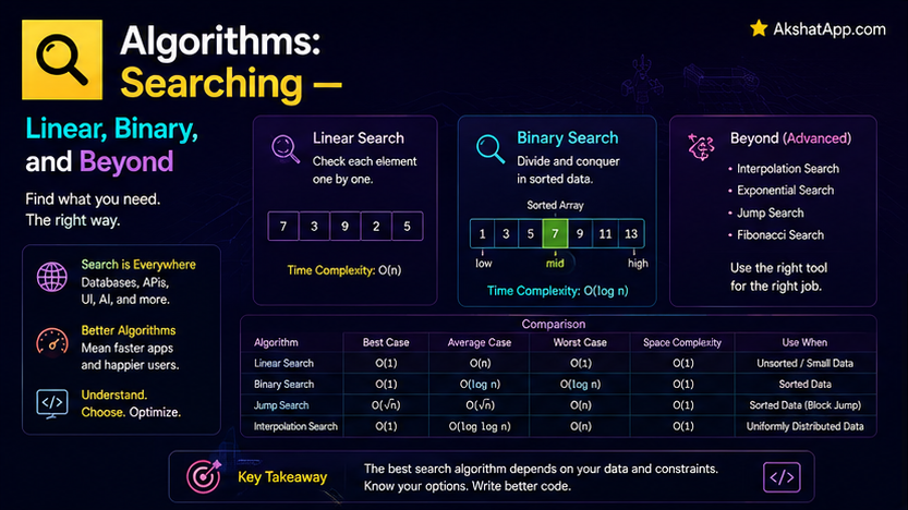
Post #8 covered how to sort a list efficiently, without fully justifying why that effort is worth spending in the first place. This post is that justification, made concrete: sorted data unlocks a search strategy dramatically faster than checking every element one at a time — the exact same halving strategy that made Post #5’s binary search tree efficient, now applied directly to a plain, sorted array.
Linear Search: The Baseline
Check every element, one at a time, until you find a match or run out of elements.
def linear_search(items: list, target) -> int:
    for i, item in enumerate(items):
        if item == target:
            return i
    return -1

print(linear_search([5, 2, 8, 1, 9], 8))  # 2
Using Post #7’s notation: O(n) — in the worst case, every single element must be checked. This works on data in any order, sorted or not, which is a genuine and sometimes overlooked advantage.
Binary Search: Requires Sorted Data, Delivers O(log n)
Binary search only works on sorted data — this is a hard requirement, not a preference — but in exchange, it delivers a dramatic improvement: check the middle element, and if it is not the target, you know immediately which entire half of the remaining data to discard, exactly as Post #5’s binary search tree eliminates half the remaining tree with every comparison.
def binary_search(sorted_items: list, target) -> int:
    low, high = 0, len(sorted_items) - 1

    while low <= high:
        mid = (low + high) // 2
        if sorted_items[mid] == target:
            return mid
        elif sorted_items[mid] < target:
            low = mid + 1   # target must be in the right half
        else:
            high = mid - 1   # target must be in the left half

    return -1

print(binary_search([1, 2, 5, 8, 9], 8))  # 3
Using Post #7’s notation: O(log n) — the identical complexity class as Post #5’s balanced BST search, arrived at through the identical underlying mechanism (eliminate half the remaining data with every comparison), just applied directly to a sorted array instead of a tree structure. The concrete payoff of this complexity class, made vivid: searching a sorted list of one billion items takes at most about 30 comparisons — not a million, not a thousand, thirty — a genuinely striking demonstration of Post #7’s growth-rate table applied to a real, human-scale example.
The Sort-Then-Search Tradeoff
If you only need to search a dataset once, sorting it first (Post #8’s O(n log n)) purely to then run one O(log n) binary search is more total work than a single O(n) linear search — sorting’s own cost dominates.
Sorting first genuinely pays off specifically when you will search the same dataset many times. The one-time sorting cost gets amortized across every subsequent search, each of which is now O(log n) instead of O(n) — for a dataset searched repeatedly, this tradeoff overwhelmingly favors sorting once, upfront.
# Searched once: linear search is simpler and comparably fast
result = linear_search(unsorted_data, target)

# Searched many times: sort once, then binary search repeatedly
sorted_data = sorted(unsorted_data)  # O(n log n), paid once
for target in many_search_targets:
    result = binary_search(sorted_data, target)  # O(log n) each, many times
Searching Across Every Structure Covered in This Series
| Structure | Search Complexity | Requires Sorted/Special Structure? |
|---|---|---|
| Unsorted array (Post #3) | O(n) | No |
| Sorted array | O(log n) | Yes — sorted |
| Linked list (Post #3) | O(n) | No |
| Hash table (Post #4) | O(1) average | No — but requires exact key |
| Balanced BST (Post #5) | O(log n) | Yes — BST ordering property |
This table is genuinely the payoff of this entire series so far — every structure’s search performance, now expressed precisely using Post #7’s notation, directly comparable for the first time. The practical decision this table supports: if you need fast lookup by an exact key and do not need sorted-order traversal, Post #4’s hash table wins outright at O(1). If you need sorted-order traversal and fast search, Post #5’s balanced BST is the right structure. If your data is naturally array-shaped and searched repeatedly, sorting once and binary-searching repeatedly is the right approach.
Real-World Use Cases
Dictionary and phone book lookups: The original, intuitive real-world binary search — flipping to roughly the middle, then narrowing based on alphabetical comparison, is precisely this algorithm performed by hand.
Database range queries: Many database indexes, covered fully once Post #14 addresses databases directly, rely on sorted structures specifically to enable fast binary-search-like lookups.
Version control bisection: Tools that find which specific commit introduced a bug by testing the midpoint of a range of commits, narrowing based on pass/fail, are directly applying binary search to a real, practical debugging problem.
Autocomplete and prefix matching: Sorted data structures combined with binary-search-adjacent techniques underlie many fast text-matching and autocomplete features.
Common Mistakes and Gotchas
⚠️ Mistake 1: Running binary search on unsorted data
binary_search([5, 2, 8, 1, 9], 8) # WRONG — undefined, unreliable behavior on unsorted data!This is the single most important warning in this post — binary search’s entire correctness depends on the sorted-order guarantee; running it on unsorted data can silently return an incorrect result (not necessarily an error) since the algorithm’s “discard half the remaining data” logic assumes an ordering that isn’t actually present.
⚠️ Mistake 2: Off-by-one errors in the low/high/mid boundary logic
Binary search’s boundary conditions (low <= high, mid + 1, mid - 1) are a famously easy place to introduce subtle bugs — a genuinely worthwhile exercise is tracing through this post’s implementation by hand on a small example before trusting a modified version.
⚠️ Mistake 3: Sorting data purely for a single search Covered directly above — the sort-then-search tradeoff only favors sorting when the dataset will be searched repeatedly; a single search is better served by simple linear search.
⚠️ Mistake 4: Reimplementing binary search when a built-in tool already exists
Python’s bisect module provides tested, correct binary search functionality directly — genuinely worth using in production code, with this post’s from-scratch implementation serving the same “understand it before trusting the built-in” purpose as Post #8’s sorting coverage.
Quick Reference
# Linear search — works on any order, O(n)
def linear_search(items, target):
    for i, item in enumerate(items):
        if item == target:
            return i
    return -1

# Binary search — REQUIRES sorted data, O(log n)
def binary_search(sorted_items, target):
    low, high = 0, len(sorted_items) - 1
    while low <= high:
        mid = (low + high) // 2
        if sorted_items[mid] == target:
            return mid
        elif sorted_items[mid] < target:
            low = mid + 1
        else:
            high = mid - 1
    return -1

# Python's built-in, tested binary search tools
import bisect
index = bisect.bisect_left(sorted_items, target)
The rule: unsorted or searched once → linear search. Sorted (or worth sorting because searched repeatedly) → binary search.
Exercises
Exercise 1 — Direct application
Trace through binary_search([1, 3, 5, 7, 9, 11, 13], 11) by hand, writing out the value of low, high, and mid at each iteration, before running the code to confirm your trace.
Exercise 2 — Slight variation
Modify binary_search to return the correct insertion point for a target value not currently in the list — where it would need to be inserted to keep the list sorted — rather than returning -1 for a miss.
Exercise 3 — Real-world combination Write a function that takes an unsorted list and a list of many search targets, and decides — using this post’s sort-then-search tradeoff reasoning — whether to sort the data first or perform repeated linear searches, based on the number of targets relative to the data size.
Exercise 4 — Open-ended challenge
Empirically confirm this post’s “30 comparisons for a billion items” claim: write a function that counts how many comparisons binary_search actually performs, run it against sorted lists of increasing size (1,000, 1,000,000, and if your machine can handle it, 1,000,000,000 simulated via range), and compare the actual counts to log2(n).
FAQ
Q: Is binary search always the right choice for sorted data? A: For simple “is this value present, and where” queries, yes, almost always. For more complex queries (find all values in a range, find the closest value if an exact match doesn’t exist), variations on binary search or the specialized tree structures from Post #5 may be more directly suited.
Q: Why does binary search need sorted data specifically, rather than some other property? A: The core mechanism — comparing against the middle element to eliminate half the remaining data — only produces a correct elimination decision if you can reliably infer “everything smaller is to one side, everything larger is to the other,” which is precisely what sortedness guarantees and nothing else does.
Q: Can binary search be implemented recursively instead of with a while loop? A: Yes — this post’s iterative version avoids the call stack overhead recursion introduces, but a recursive version is equally valid and arguably more directly mirrors the “eliminate half, then recurse into the remaining half” logic; Post #10 covers recursion in full, including revisiting this exact tradeoff.
Q: Does Python’s built-in in operator (x in my_list) use binary search automatically?
A: No — for a plain list, in performs a linear scan (O(n)) regardless of whether the list happens to be sorted, since Python has no way to know your list is sorted without being told explicitly; use the bisect module directly, as covered in this post’s quick reference, to actually get binary search’s performance benefit.
Summary and Next Steps
You now understand exactly why Post #8’s sorting effort pays off: binary search’s O(log n) performance, arrived at through the identical halving strategy that made Post #5’s BST efficient, delivers a dramatic, concrete improvement over linear search’s O(n) — thirty comparisons instead of a billion, for a billion-item dataset. The comparison table in this post ties together every structure’s search performance covered across this entire series, precisely, for the first time.
Your next step: Complete Exercise 4 — empirically confirming the “30 comparisons for a billion items” claim — since verifying this post’s most striking claim yourself, with real code and real numbers, is what turns Big O notation from Post #7 into something you trust as genuinely, practically true rather than abstract theory.
Last updated: August 2026.
Share This Post

Join our newsletter!
Get the latest developer guides, tutorials, and tips delivered straight to your inbox.